Turbulence modeling

Turbulence modeling is the construction and use of a model to predict the effects of turbulence. Averaging is often used to simplify the solution of the governing equations of turbulence, but models are needed to represent scales of the flow that are not resolved.^[1]

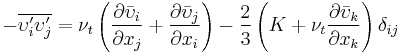
A closure problem arises in the Reynolds-averaged Navier-Stokes (RANS) equation because of the non-linear term $\overline{\upsilon_i^\prime \upsilon_j^\prime}$ from the convective acceleration, known as the Reynolds stress,

$R_{ij}=\overline{\upsilon_i^\prime \upsilon_j^\prime}$

Closing the RANS equation requires modeling the Reynold's stress $R_{ij}$ . Joseph Boussinesq was the first practitioner of this, introducing the concept of eddy viscosity. In 1887 Boussinesq proposed relating the turbulent stresses to the mean flow to close the system of equations. Here the Boussinesq hypothesis is applied to model the Reynolds stress term. Note that a new proportionality constant $\nu_t > 0$ , the turbulent eddy viscosity, has been introduced. Models of this type are known as eddy viscosity models or EVM's.

$-\overline{\upsilon_i^\prime \upsilon_j^\prime} = \nu_t\left (\frac{\partial\bar\upsilon_i}{\partial x_j}%2B\frac{\partial\bar\upsilon_j}{\partial x_i} \right )-\frac{2}{3}\left (K %2B \nu_t \frac{\partial\bar\upsilon_k}{\partial x_k} \right ) \delta_{ij}$

Which can be written in shorthand as

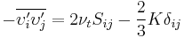
$-\overline{\upsilon_i^\prime \upsilon_j^\prime} = 2\nu_tS_{ij}-\frac{2}{3}K\delta_{ij}$

where $S_{ij}$ is the mean rate of strain tensor

$\nu_t$ is the turbulent eddy viscosity

$K = \frac{1}{2}\overline{\upsilon_i^{\prime\, 2}}$ is the turbulent kinetic energy

and $\delta_{ij}$ is the Kronecker delta.

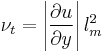
In this model, the additional turbulent stresses are given by augmenting the molecular viscosity with an eddy viscosity.^[2] This can be a simple constant eddy viscosity (which works well for some free shear flows such as axisymmetric jets, 2-D jets, and mixing layers). Later, Ludwig Prandtl introduced the additional concept of the mixing length, along with the idea of a boundary layer. For wall-bounded turbulent flows, the eddy viscosity must vary with distance from the wall, hence the addition of the concept of a 'mixing length'. In the simplest wall-bounded flow model, the eddy viscosity is given by the equation:

$\nu_t = \left|\frac{\partial u}{\partial y}\right|l_m^2$

where:

$\frac{\partial u}{\partial y}$ is the partial derivative of the streamwise velocity (u) with respect to the wall normal direction (y);

$l_m$ is the mixing length.

This simple model is the basis for the "Law of the Wall", which is a surprisingly accurate model for wall-bounded, attached (not separated) flow fields with small pressure gradients.

More general turbulence models have evolved over time, with most modern turbulence models given by field equations similar to the Navier-Stokes equations.

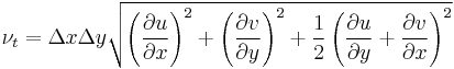
Among many others , Joseph Smagorinsky (1964) proposed a useful formula for the eddy viscosity in numerical models, based on the local derivatives of the velocity field and the local grid size:

$\nu_t = \Delta x \Delta y \sqrt{\left(\frac{\partial u}{\partial x}\right)^2 %2B \left(\frac{\partial v}{\partial y}\right)^2 %2B \frac{1}{2}\left(\frac{\partial u}{\partial y} %2B \frac{\partial v}{\partial x}\right)^2}$

The Boussinesq hypothesis is employed in the Spalart-Allmaras (S-A), k-ε (k-epsilon), and k-ω (k-omega) models and offers a relatively low cost computation for the turbulent viscosity $\nu_t$ . The S-A model uses only one additional equation to model turbulent viscosity transport, while the k models use two.

Common Models

The following is a list of commonly employed models in modern engineering applications.

Spalart–Allmaras (S-A)
k-ε (k-epsilon)
k-ω (k-omega)
SST (Menter’s Shear Stress Transport)

References

^ Ching Jen Chen, Shenq-Yuh Jaw (1998), Fundamentals of turbulence modeling, Taylor & Francis, http://books.google.co.uk/books?id=HSCUGJ1n8tgC
^ John J. Bertin, Jacques Periaux, Josef Ballmann, Advances in Hypersonics: Modeling hypersonic flows, http://books.google.co.uk/books?id=edy-vDzifvAC&pg=PA6